Modeling microbial fermentation with XGBoost

Fermentation is essential in food production. Dough, cheese, yogurt, kombucha, and many other foods rely on the growth of microorganisms such as yeasts and lactic acid bacteria. Their growth is sensitive to several factors:

Temperature
Sugar and salt concentrations
pH level
Inoculum, or microbial quantity at the start
Time

However, modeling fermentation is challenging:

Real-world data is scarce and noisy.
Experiments are time-consuming.
The system is nonlinear and complex.

To tackle this, I used XGBoost, a high-performance implementation of gradient boosting. Rather than fitting a single model, XGBoost builds an ensemble of simple decision trees that iteratively correct each other’s errors.

This approach excels at capturing nonlinear effects and variable interactions while remaining robust to noisy, low-volume datasets, making it well suited to experimental fermentation settings. It also provides useful insights into which variables matter most, which is crucial when working with biological systems.

In this article, I’ll show how I simulated microbial fermentation data, trained an XGBoost model, and explored how different parameters impact final microbial density.

Simulating a fermentation dataset

In microbiology, cell growth often follows a sigmoid-shaped curve. One of the most common formulations is the logistic growth equation:

N(t) = \frac{N_{\max}}{1 + \exp\left[-k(t-t_m)\right]}

Where:

$N(t)$ is microbial population, in log CFU/mL, at time $t$ .
$N_{\max}$ is maximum population density.
$k$ is growth rate.
$t_m$ is time when growth rate reaches its peak.

This equation produces a slow start, an exponential phase, and a plateau, just like real fermentation.

What influences growth?

I made $N_{\max}$ , $k$ , and $t_m$ dependent on input variables to simulate biological behavior:

Variable	Simulated range
Temperature	15–45°C
Sugar concentration	10–100 g/L
Salt concentration	0–5%
Initial pH	4.5–6.5
Inoculum	5–9 log CFU/mL
Fermentation time	6–48 hours

To simulate natural experimental noise, I added Gaussian noise with mean 0 and standard deviation 0.2.

Dataset simulation

import numpy as np
import pandas as pd

np.random.seed(42)
n = 1000

# Input variables
temperature = np.random.uniform(15, 45, n)
sugar = np.random.uniform(10, 100, n)
salt = np.random.uniform(0, 5, n)
initial_pH = np.random.uniform(4.5, 6.5, n)
inoculum = np.random.uniform(5, 9, n)
time = np.random.uniform(6, 48, n)

# Growth parameters
k = 0.1 + 0.05 * ((temperature - 30) / 10) - 0.03 * salt
k = np.clip(k, 0.01, 0.3)
N_max = 9 + 0.01 * sugar - 0.05 * salt
N_max = np.clip(N_max, 7, 12)
t_m = 24 - 0.5 * (inoculum - 5)

# Logistic growth with noise
N_t = N_max / (1 + np.exp(-k * (time - t_m)))
N_t += np.random.normal(0, 0.2, size=n)
N_t = np.clip(N_t, 5, 12)

# Final dataset
df = pd.DataFrame({
    "temperature": temperature,
    "sugar": sugar,
    "salt": salt,
    "initial_pH": initial_pH,
    "inoculum": inoculum,
    "time": time,
    "final_density": N_t
})

print(df.head())

Dataset sample:

	temperature	sugar	salt	initial_pH	inoculum	time	final_density
0	26.236204	26.661964	1.308528	5.845406	7.287984	22.532692	5.000000
1	43.521429	58.771085	1.234894	6.093363	8.221729	25.884298	5.925936
2	36.959818	88.565125	4.531273	5.000936	8.040644	41.890991	5.355006
3	32.959755	75.900240	1.247731	5.749748	5.615600	20.280184	5.000000
4	19.680559	82.590503	1.359749	5.643492	5.596998	42.525287	5.178634

Training an XGBoost model

We now train a model to predict final_density from all input variables.

from sklearn.metrics import mean_squared_error
from sklearn.model_selection import train_test_split
from xgboost import XGBRegressor

X = df.drop(columns=["final_density"])
y = df["final_density"]

X_train, X_test, y_train, y_test = train_test_split(
    X,
    y,
    test_size=0.2,
    random_state=42
)

model = XGBRegressor(objective="reg:squarederror", n_estimators=100)
model.fit(X_train, y_train)

y_pred = model.predict(X_test)
rmse = np.sqrt(mean_squared_error(y_test, y_pred))
print(f"Baseline RMSE: {rmse:.3f}")

Evaluation with RMSE

I use Root Mean Squared Error, or RMSE, as evaluation metric:

\operatorname{RMSE} = \sqrt{\frac{1}{n}\sum_{i=1}^{n}(y_i-\hat{y}_i)^2}

If RMSE is 0.259, model predictions differ from observed values by approximately 0.259 log CFU/mL on scale measured by this error metric. This is a good result considering model simplicity and intentionally noisy data.

Feature importance

import matplotlib.pyplot as plt
from xgboost import plot_importance

plot_importance(model)
plt.title("Feature Importance")
plt.tight_layout()
plt.show()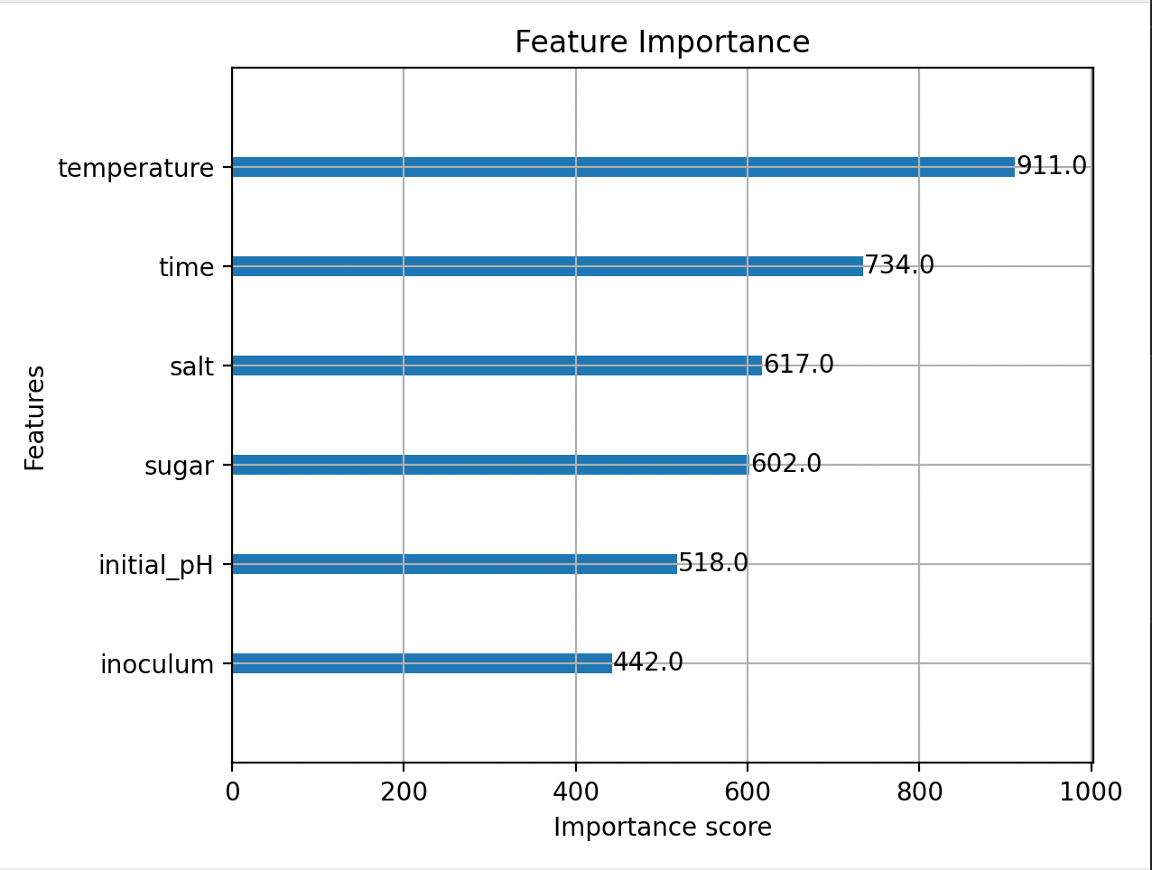

Most important variable is temperature, followed by fermentation time, salt, and sugar. This makes biological sense:

Temperature drives metabolic activity of microorganisms.
Time allows growth to reach its plateau.
Salt generally inhibits microbial growth.
Sugar provides a carbon source, although its effect saturates.

Importance scores align with microbiological principles. Temperature has highest impact on predicted outcomes, confirming its strong and known regulatory role in fermentation dynamics.

Feature importance should still be interpreted cautiously: it describes how fitted model uses variables in this simulated dataset, not universal biological causality.

Predictions versus ground truth

import matplotlib.pyplot as plt
import numpy as np
from sklearn.metrics import mean_squared_error

y_pred = model.predict(X_test)
rmse = np.sqrt(mean_squared_error(y_test, y_pred))

plt.figure(figsize=(6, 6))
plt.scatter(y_test, y_pred, alpha=0.5)
plt.plot([5, 12], [5, 12], "--", color="gray")
plt.xlabel("True")
plt.ylabel("Predicted")
plt.title("Predictions vs Actual Values")
plt.grid(True)
plt.tight_layout()
plt.show()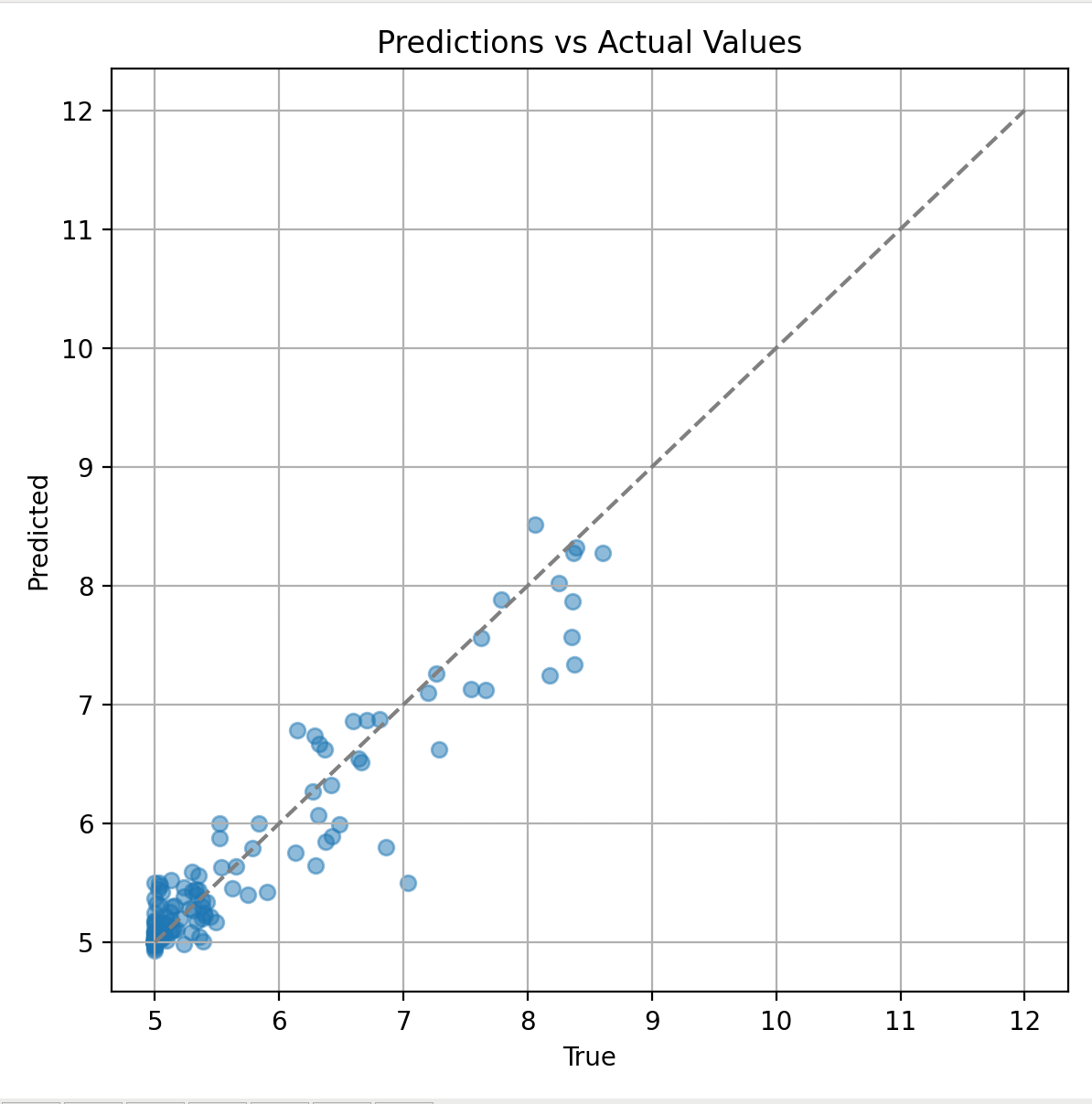

Scatter plot comparing predicted and actual microbial densities against a diagonal reference line — Baseline predictions against simulated ground-truth microbial densities.

Scatter plot shows dense clustering of predictions between 5.0 and 6.5 log CFU/mL, tightly aligned along diagonal. This indicates strong model performance in moderate growth range, where biological responses are more predictable.

For higher microbial densities above 7.5, predictions become more scattered and deviate from diagonal. Possible reasons include:

Increased biological variability in high-activity scenarios
Limits of features used
Greater sensitivity to noise in extreme regions

In practice, fermentations with extremely high activity can exhibit nonlinear dynamics that are difficult to capture without richer features or mechanistic modeling.

Improving the model

Feature engineering

df["sugar_per_hour"] = df["sugar"] / df["time"]
df["temp_salt_ratio"] = df["temperature"] / (df["salt"] + 1)
df["growth_potential"] = (df["temperature"] - 30) * (df["sugar"] - df["salt"])

X = df.drop(columns=["final_density"])
y = df["final_density"]

X_train, X_test, y_train, y_test = train_test_split(
    X,
    y,
    test_size=0.2,
    random_state=42
)

These features combine key inputs and express domain knowledge more explicitly.

Hyperparameter tuning

model = XGBRegressor(
    objective="reg:squarederror",
    n_estimators=300,
    max_depth=4,
    learning_rate=0.05,
    subsample=0.8,
    colsample_bytree=0.8,
    reg_lambda=1.0,
    reg_alpha=0.1
)

model.fit(X_train, y_train)
y_pred = model.predict(X_test)
improved_rmse = np.sqrt(mean_squared_error(y_test, y_pred))

This configuration uses smaller learning steps, more trees, regularization, and subsampling to reduce overfitting and improve generalization.

Results after improvements

Improved RMSE: 0.2 log CFU/mL

This is approximately 23% reduction in error compared with baseline.

Updated feature importance

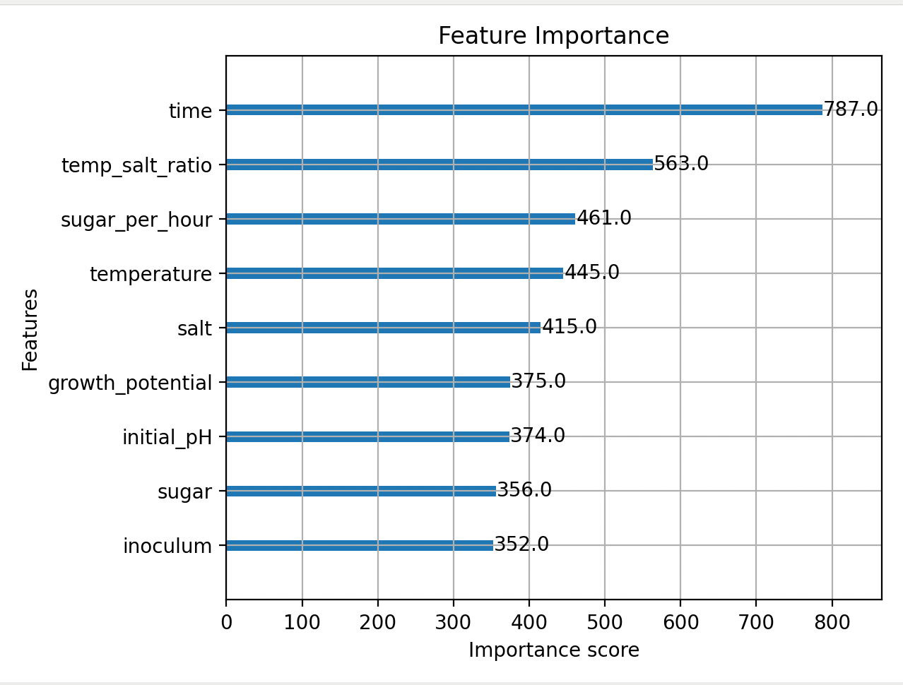
New engineered features such as temp_salt_ratio and sugar_per_hour now rank above temperature and sugar, indicating that domain-specific transformations better capture effects of combined variables.

Updated XGBoost feature importance plot led by time, temperature-to-salt ratio, and sugar per hour — Feature importance after adding domain-informed variables and tuning model.

Updated scatter plot comparing predicted and actual microbial densities against a diagonal reference line — Predictions after feature engineering and hyperparameter tuning.

Updated prediction plot

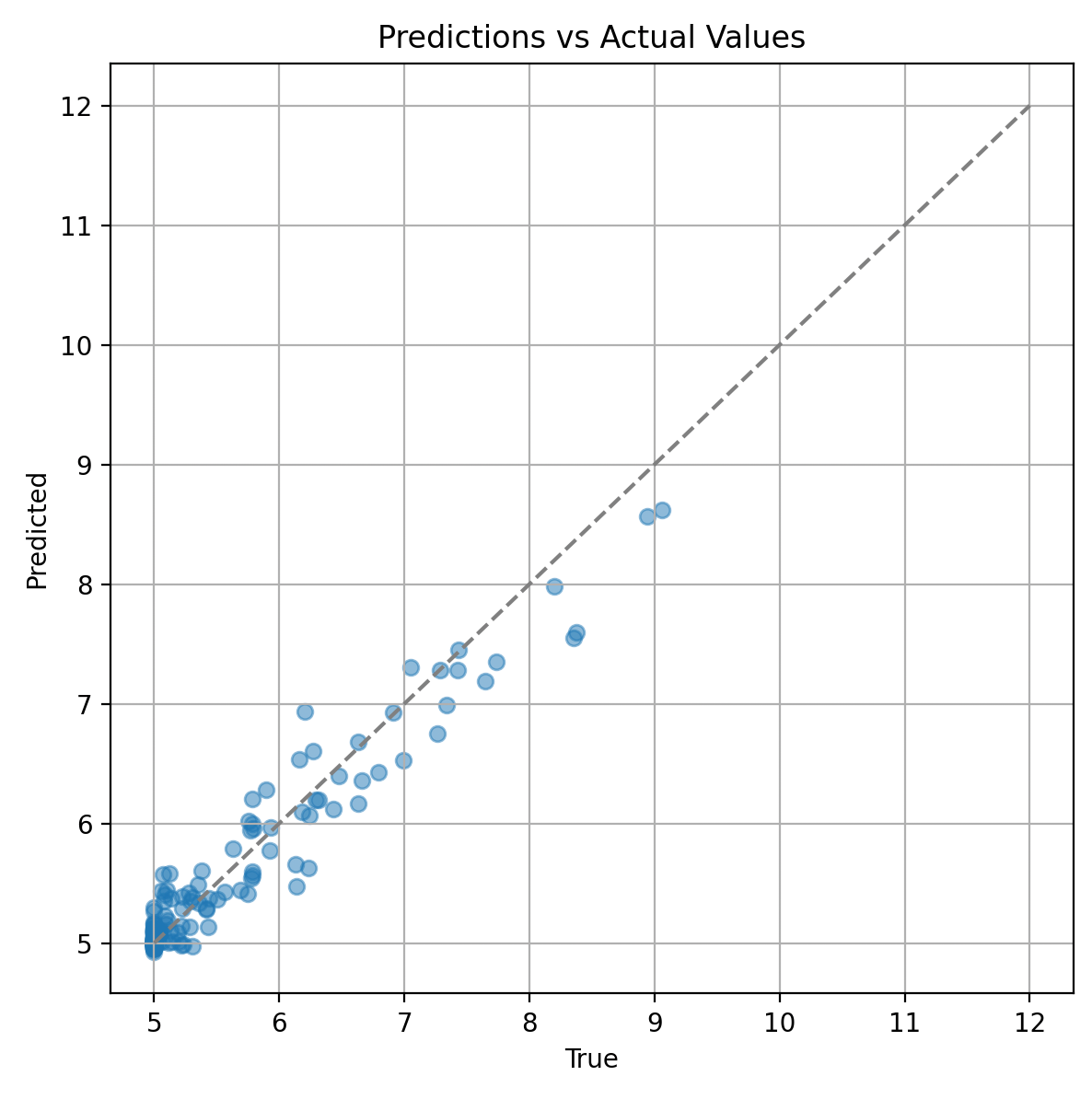
New scatter plot shows predictions more tightly clustered around diagonal, with reduced variance at higher densities. This indicates better generalization across broader range of simulated biological behavior.

Limits of this experiment

This workflow demonstrates modeling process on synthetic data. Reported performance measures recovery of relationships deliberately encoded in simulator; it does not validate performance on real fermentation experiments. Real applications require independent experimental data, appropriate validation design, uncertainty analysis, and careful control of biological and measurement variability.

Key takeaways

Machine learning can model simulated biological systems, even with noisy data.
Feature engineering plays a critical role in capturing complex interactions.
Hyperparameter tuning can produce meaningful performance gains.
Metrics and visualizations such as RMSE and prediction plots are essential for validation.
Strong performance on simulated data does not replace validation on real fermentation data.

Abstract